
The Normalization Expectation. The global financial crisis, resulting deep recession, and domination by policymakers the last five years have been anything but normal for the markets. If we were to anthropomorphize this period, we might borrow the late, great, Marty Feldman’s line and name it “Abby Normal.”[i] In the latest adventures of Abby, in May of last year the Fed started to change its projection of the path of monetary policy.
A critical assumption for this change is the view that, over the next few years, key measures of the U.S. economy will approach levels close to long-run projections. Call it “Normie Normal” if you will. The FOMC projects[ii] the annual pace of GDP growth over the next two years to be 3.1%. That would be right on the 50-year average, and above the committee’s projection of a 2.3% long-run average growth rate.[iii] Out in 2016, the FOMC projects 2.9% GDP growth, a 1.9% inflation rate, and a Q4 unemployment rate of 5.6%. Plugging in these various figures, the committee’s projections imply that excess slack in the economy, as measured by the nominal output gap, would approach zero by the end of 2016.
Private sector economists jumped on the Fed bandwagon, at least for the 2014 outlook, as the trend of positive economic surprises continued and the level of fiscal policy uncertainty receded.[iv] The December Blue Chip forecaster consensus for 2014 GDP growth was 2.8%, just a few ticks under the FOMC projection. Movements in financial markets also reflect expectation for a normalizing economy. Last year, financial markets transitioned from being driven mainly by the yield/return chase orchestrated by the Fed to being still chase-driven, but also propelled by an improved outlook.
Once a year over the last few years markets got going on this “escape velocity” or ”normalization” hand and played it until something big (e.g., adverse fiscal policy and the euro crisis) forced it to fold the cards on that outlook and rely on central bank easing to keep going. So here we are again, with markets playing that same hand. Now, recent actions on the Hill in light of the upcoming elections have removed the government shutdown joker from the deck. A debt ceiling debacle seems out of play. The euro area joker can always pop up, but we haven’t seriously seen it since the summer of 2012. That’s long enough for markets to effectively forget. The China joker remains in the deck. Central banks may fumble policy communications or make policy mistakes. These are well-acknowledged macro risks. Any adverse true surprises for markets this year will come from elsewhere. To paraphrase Donald Rumsfeld, we know we do not know from where these surprises may come.
So, we start the year with the expectation that the U.S. economy is nicely along the path to normalization, the consensus outlook from the central bank and private forecasters. Higher long-term interest rates, tighter high-yield bond spread, and rallying equities are evidence that the markets are on board. An early challenge in 2014 will be if markets already have priced in the normalization expectation and so are ahead of reality. There is some evidence of this:
- Equity valuations are no longer cheap.
- The ten-year T-note yield is almost twice the low from last May.
- Credit spreads to Treasury are at summer 2007 levels.
- The level of expected equity price volatility is quite low.
- The yield curve has a more normal (concave) shape from the three-year point on out.[v]
It seems this normalization expectation led to a rediscovery of the Goldilocks-like scenario that excites markets. A Goldilocks belief in moderate growth with low inflation, at a time of near-zero savers rates, would lead investors to continue to favor riskier assets. In that case, sentiment probably will not suffer even if traditional valuations of riskier assets (such as P/Es and spreads to Treasury) become quite extended. It is about escaping zero-percent savers rates and riding momentum. “Adaptive expectations” in street translation means that many investors will chase recent trends and past performance. While typically very aware that this is their behavior, they rationalize it because they think they can get out before the top. Some call it the “Greater Fool” theory. Others refer to it as beating everybody out of the pool. One thing for sure, the behavior is a hardy perennial.
Will this behavior become a problem in 2014? Will the markets move into the late innings of the greatest yield/return chase of them all? This will greatly depend on market perceptions of, and reactions to, Fed communications in light of the data results. The normalization/Goldilocks scenario should persist if the economic data remain solid, but not so strong that it would force the Fed to accelerate its timetable for a rate hike.
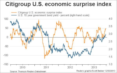
In the near-term, the trend of positive economic data surprises since the Draghi pledge of July 2012 (see the surprise index series that fluctuates within the red lines in Chart 1[vi]) is extended. It therefore makes sense for the data results eventually to start to undershoot recently improved economic forecasts. A developing trend of negative economic surprises would keep the FOMC from increasing the pace of the QE taper or softening the wording of the forward guidance. Currently the Fed has markets expecting a near-zero policy rate into mid-2015. But this expectation is subject to change and really depends on the data. As long as savers rates remain near zero, and are expected to remain there, the party ought to continue.
Chart 1: The Trend of Positive Economic Surprises Is Extended
Fixed Income Workshop: Useful Measurements. In the first two Fixed Income Workshops, we discussed the basic components of a bond’s total return and the limitations of the classic duration measures in explaining and predicting fixed income performance. We also discussed the more recent generation of duration measures that help decompose a portfolio into useful summary components measuring exposure to pure interest rate movement, yield curve twists, and spread changes. These are often viewed against a benchmark to offer a reasonable basis for evaluating performance results or predicting future performance. This week, let’s review some useful measures to evaluate portfolio returns earned and the volatility of returns experienced.
The classic total return measure ultimately is the most important to the investor because it is actually what happened, before taxes, to the invested money. But by itself it tells us nothing about the story behind the result. Investors may compare a bond or bond portfolio return to several measures such as equity returns, risk-free T-bill yield, and the inflation rate. That comparison helps deepen understanding but still lacks information about the volatility experienced on the road to that return, i.e. how bumpy the ride was to earn the reward.
In March 1952, Harry Markowitz published a paper in the Journal of Finance that laid the foundation for the classic risk/reward measures used today. This was where the first discussion of expected return and its variance can be found. By the early 1960s, a number of researchers had added onto Markowitz’s work and those measures, such as the Sharpe and Treynor ratios, are standard in any summary of portfolio performance. In 1973, Black and Scholes applied these ideas to the pricing of options and thus was born the modern derivatives markets. (But that is another, and fascinating, story.) Let’s briefly summarize some classic and useful measures of a portfolio’s return and return volatility.
-
Total Return. Total return is the whole ball of wax; some might say it is the sum of the risk-free rate, the return attributable to the market (beta) and the return attributable to manager actions (alpha). The nominal total return is not adjusted for inflation whereas the real total return is. When measured over annualized timeframes, the geometric, not arithmetic, return is calculated.
-
Excess Return. This is the difference between the return earned on a portfolio and the return of its benchmark. The term “excess return” is a bit misleading because the figure can be negative, too. Excess return is sometimes called the alpha component.[i] In fixed income portfolio analysis, the excess return can be based on a standard benchmark such as the Barclay’s Aggregate Index or an option-adjusted duration-matched benchmark.
-
Variance and Standard Deviation. These measures were developed in the 1860s by Francis Galton, also the father of regression and correlation.[ii] Variance is a standardized measure of return fluctuations over a given timeframe. The standard deviation simply transforms the variance into a figure that can be directly compared with the nominal return.[iii] It is very useful and elegant. A standard deviation around the mean represents 68% of a two-tailed normal distribution of a sample data set while 95% of the normal distribution is covered by two standard deviations.
-
Tracking Error. How much did portfolio returns fluctuate compared to the benchmark? Tracking error is typically measured by the standard deviation of the excess return data series. Large tracking error suggests that the portfolio did not behave much like the benchmark over the timeframe. This is a bigger deal when using a benchmark replication strategy, wherein a minimal tracking error is desired.
-
R-squared. This is another measure of how closely a portfolio tracked a benchmark. It is formally called the coefficient of determination and also written as “R2.” It is the square of the sample correlation coefficient (called “R”). R-squared gives the percentage of historical movement of portfolio returns that is explained by the movement in the benchmark. For example, assume that measured over three years, the R-squared for portfolio Y is 70%. We can state that over those three years, 70% of the movement of the returns on portfolio Y is explained by the movement in the returns for benchmark X.
-
Sharpe Ratio. For a given timeframe, this is the portfolio average total return minus the risk-free return divided by the standard deviation of the total returns. For example, assume a 7% portfolio return, 2% risk-free return and 6% standard deviation. The Sharpe Ratio is 7% minus 2% then divided by 6% which equals 0.83 units of return earned per unit volatility experienced. This measure is little good if used in isolation, so the ratio is compared to ratios for a benchmark, other markets, and competing products. Compared to a competitor product with a 0.50 Sharpe Ratio, the example investor product 0.83 Sharpe Ratio would provide evidence of more return earned per unit of return volatility experienced.
-
Information Ratio. This measure is a refinement of the Sharpe Ratio by using the Excess Return series. It is the ratio of the average excess return to the standard deviation of the excess returns (i.e., the tracking error). The refinement here is that we are measuring the return over/under the benchmark which allows us to better measure the individual manager’s success. This ratio is interpreted as the unit of excess return earned per unit of excess return volatility experienced over a given timeframe. For example, if over three years a portfolio had an average annual excess return of 3% with a standard deviation of 2% for the excess returns, the information ratio would be 1.5 units of excess return per unit of return volatility experienced. This is a useful measure when comparing performance to active and passive competing products.
- Probability of Outperformance. The Information Ratio can be used to generate a statistic that gives the probability of outperformance (i.e., positive excess return) against a benchmark.[iv] To do this, we assume that the Information Ratio is normally distributed with a standard deviation of one. For example, assume a mean annualized Information Ratio over three years of positive 0.5. We next apply the “normsdist” function in Excel to the information ratio = normsdist(0.5) to calculate a result of 0.69, or a 69% probability of outperforming over a year. The probability of underperforming is one minus the probability of outperforming, or 31%[v]. The more positive the Information Ratio, the greater the probability, based on historical results, of outperforming the benchmark. Past performance undistinguishable from a benchmark would imply a 50% probability of outperformance. A negative Information Ratio (due to a negative average excess return) would mean a lower than 50% probability of outperformance versus the benchmark. For example, a negative 0.6 Information Ratio gives a 27% probability of outperformance. As with all historically-based analysis, it is important to use several timeframes and compare the results.
Words of Caution. To use these statistical tools, one must assume the sample data are normally distributed. In fact, this is the critical assumption in parametric statistics. There are problems with the predictive power of the statistics when the data series (i.e., the real world) starts to behave quite differently compared to the past (e.g., credit spreads during the financial crisis). But in quieter times it works nicely enough. The less normally-distributed the sample data, the less predictive power of the statistics generated.[vi]
CIM Outlook. We expect the economy to experience some drag from restrictive fiscal policy in an environment of dysfunctional federal governance. The risk of a strong adverse shock from fiscal policy in 2014, however, has been mitigated because of the coming November mid-term elections. The economy is in a sub-par economic expansion and not fully recovered from the severe financial crisis. We expect the economy to tend to post sub-trend growth rates with low inflation and an improving but soft labor market. For full-year 2014, there is a reasonable chance the rate of GDP growth could fail to reach 2.5%, below the 50-year average of 3.1%, but there is reason to be more optimistic than in recent years. The output gap, however, will take at least two years to close under the FOMC’s generally optimistic forecast.
Under the Janet Yellen-led Fed, we expect monetary policy to continue on the same general course set under Ben Bernanke. Next year, two Board of Governors seats must be filled and a new Vice Chair appointed.[vii] That process will be easier after the recent change in Senate filibuster rules and the appointees should be Yellen policy allies. On the other hand, there will be two policy-voting hawks on the FOMC in 2014 versus one this year. As a result, we could see two dissenting votes on FOMC decisions in 2014. The Fed’s December decision to taper could tame the hawks for a while. We might, however, see a policy-dove dissent in 2014 as occurred with the December FOMC decision.
Given our outlook that economic growth should be somewhat adversely influenced by federal fiscal restraint, and with the economy still experiencing excess capacity, we expect tapering of QE3 to occur slowly over the course of 2014. The Fed will continue to signal to markets, through strengthened forward guidance, to expect a first hike in the policy target rate no earlier than later in 2015 and possibly in 2016. It would take a financial crisis or convincing evidence of a recession and/or deflation threat for the Fed to re-accelerate the QE or engage in another form of easing.
[i] More traditionally, what is termed alpha is the constant term, or Y intercept, while beta is the x variable coefficient (i.e., the slope of the line) in the equation Y = a + bX +e. “e” is the regression standard error term.
[ii] As well as other measures we had to grind out on paper with aid of an LED Texas Instruments calculator in the 1970s. At least we arrived after slide rules.
[iii] The variance is the mean of squared differences between the observations and the mean. Standard deviation is the square root of the variance.
[iv] Source: https://www.riskprep.com/component/exam/?view=exam&layout=detail&id=52
[v] Or insert a negative sign for a positive information ratio and vice versa in the normsdist function.
[vi] One should measure the skew and kurtosis of the sample distribution to see if it approaches a normal shape allowing for comfortable use of parametric statistical projections.
[vii] Stanley Fischer is reported to be President Obama’s nominee for Vice Chair.
[i] As spoken by Feldman’s Igor in Mel Brooks’ Young Frankenstein. http://www.youtube.com/watch?v=yH97lImrr0Qhttp://oldhollywood.tumblr.com/post/7353971697/marty-feldman-abby-normal-in-young
[ii] Projections for GDP growth and the unemployment and inflation rates are the midpoints of the FOMC SEP central tendency range.
[iii] By the way, in the wake of the financial crisis, and in light of demographic trends, the FOMC has consistently lowered its estimate of the long-run GDP growth rate.
[iv] The consensus for GDP growth drag from fiscal policy in 2014 is estimated to be 0.4 point compared to 1.5 points in 2013. This does not account for a few ticks of additional drag that should result if Congress does not retroactively extend expired unemployment benefits.
[v] Broad measures of the slope, however, remain quite steep, thanks to the Fed’s near-ZIRP.
[vi] As our own Matt Duch noted, this chart shows a compression of the range of economic data surprises in recent years. This makes sense as we move farther from the great recession and historically weak recovery toward a less abnormal economy. Forecasts have become less inaccurate.


