
It’s impossible to build an investment plan without estimating returns. This estimate of returns determines your need to take risk—how high an allocation to equities you will need to reach your goal.
If your estimate is too high, it’s likely you won’t have sufficient assets to reach your retirement goal. If it’s too low, it could lead you to allocate more to equities, taking more risk than necessary. Alternatively, it could lead you to lower your goal, save more or plan on working longer. Despite its importance, there is much disagreement about how to estimate stock returns.
Research on the expected equity premium, including Aswath Damodaran’s 2022 paper “Equity Risk Premiums (ERP): Determinants, Estimation and Implications,” has found that the best predictor of future equity returns is current valuations—using measures such as the earnings yield (E/P) derived from the Shiller CAPE 10 (or for that matter, the CAPE 7, 8 or 9) or the current E/P—not historical returns. A review of the evidence led Damodaran to conclude: “Equity risk premiums can change quickly and by large amounts even in mature equity markets. Consequently, I have forsaken my practice of staying with a fixed equity risk premium for mature markets, and I now vary it year to year, and even on an intra-year basis, if conditions warrant.”
Damodaran’s approach is similar to the one we use at Buckingham. At the beginning of each year, we estimate returns for all asset classes and then use those estimates in our assumptions when running Monte Carlo simulations. While our methodology has changed somewhat over time, our forecast for equities has always been based on current valuations, not historical returns. Today, we take the average of the estimate using the Shiller CAPE 10 E/P and the Gordon Growth Model (also known as the dividend discount model). For factors other than market beta (such as size and value), we have chosen to give the historical premium a one-third haircut based on research showing that some degradation of premiums, even risk-based ones, occurs post-publication. That, in turn, helps us determine the most appropriate asset allocation for clients.
We have been following this process since 2003. I thought it would be an interesting exercise to evaluate the accuracy of our forecasts. Before digging into the results, it’s important to understand that investors should treat all estimates of returns to risky assets only as the mean of what is potentially a wide dispersion of returns. In other words, it’s unlikely you will earn the mean estimated return. That is why we use Monte Carlo simulations to help us determine the most appropriate asset allocations—expected returns are not deterministic, but probabilistic. For example, let’s consider the results from Cliff Asness’ study on the Shiller CAPE 10’s ability to forecast future returns.
In a November 2012 paper, “An Old Friend: The Stock Market’s Shiller P/E,” Asness, of AQR Capital Management, found that the Shiller CAPE 10 does provide valuable information. Specifically, he found 10-year-forward average real returns dropped nearly monotonically as starting Shiller P/Es increased. He also found that as the starting Shiller CAPE 10 ratio increased, worst cases became even worse and best cases became weaker.
However, while the metric provided some valuable insights, there were still very wide dispersions of returns. For instance:
When the CAPE 10 was below 9.6, 10-year-forward real returns averaged 10.3%. In relative terms, that is more than 50% above the historical average of 6.8% (9.8% nominal return less 3.0% inflation). The best 10-year-forward real return was 17.5%. The worst 10-year-forward real return was still a respectable 4.8%, just 2.0 percentage points below the average and 29.0% below it in relative terms. The range between the best and worst outcomes was a 12.7 percentage point difference in real returns.
When the CAPE 10 was between 15.7 and 17.3 (about its long-term average of 16.5), the 10-year-forward real return averaged 5.6%. The best and worst 10-year-forward real returns were 15.1% and 2.3%, respectively. The range between the best and worst outcomes was a 12.8 percentage point difference in real returns.
When the CAPE 10 was between 21.1 and 25.1, the 10-year-forward real return averaged just 0.9%. The best 10-year-forward real return was still 8.3%, above the historical average of 6.8%. However, the worst 10-year-forward real return was now -4.4%. The range between the best and worst outcomes was a difference of 12.7 percentage points in real terms.
When the CAPE 10 was above 25.1, the real return over the following 10 years averaged just 0.5%—virtually the same as the long-term real return on the risk-free benchmark, one-month Treasury bills. The best 10-year-forward real return was 6.3%, just 0.5 percentage points below the historical average. But the worst 10-year-forward real return was now -6.1%. The range between the best and worst outcomes was a difference of 12.4 percentage points in real terms.
What can we learn from the preceding data? First, starting valuations matter—a lot. Higher starting values mean that not only are future expected returns lower (and vice versa), but the best outcomes are lower and the worst outcomes worse. However, a wide dispersion of potential outcomes, for which we must prepare when developing an investment plan, still exists—high starting valuations don’t necessarily result in poor outcomes.
It’s also why an investment plan should include a Plan B—a contingency plan that lists the actions to take if financial assets were to drop below predetermined level. Actions might include remaining in or returning to the workforce, reducing current spending, reducing the financial goal, selling a home and/or moving to a location with a lower cost of living.
Let’s turn now to Buckingham’s prior forecasts of long-term, unconditional (regardless of the horizon) expected returns. In the framework we use, an acceptable range for the expected return is one standard deviation divided by the square root of the number of years in the sample (the standard error of the mean). For example, in a nine-year period, the expected return should be within one-third of one standard deviation of the actual return.
The following table presents returns for each of the periods for which we have at least 10 years of results available. Each period ends in 2018. Over shorter periods, returns are so volatile that measuring the quality of a forecast is not as meaningful an exercise. For example, while the compound return to U.S. stocks has been about 10%, in very few years (just six of the last 97) has the return fallen between 8% and 12%. In just 20 years over the last 97 has the return fallen between 0% and 12%. With that caveat in mind, the appendix following this article shows our forecasts and the results for the years 2014 through 2018 (which gives us at least five years of returns after the estimate).
The actual returns data is based on the MSCI All-Country World Investable Market Index (IMI). As you review the results, keep in mind that the period began in 2003, when the U.S. Shiller CAPE 10 was about 23. It reached a nadir of about 14 in February 2009. As of July 18, 2023, it was about 32, 39% above the level at the start of the period. That increase provided an “unforecastable” tailwind to stock returns, helping to explain why our forecasts generally were below the actual returns.
Changes in valuation are what John Bogle called the “speculative return.” The record shows there are no good forecasters of changes in valuations, which is why we assume no change.
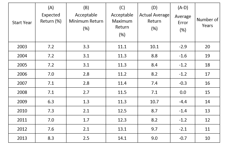
In all 11 cases the actual average returns were inside the acceptable range. To show an apples-to-apples comparison with the expected return, this analysis reflects the average returns—what an investor should expect in any given year. The annualized returns would be lower over the period due to the volatility in stock prices. The average error in absolute terms was 1.5%. And generally, the longer the period, the more accurate the forecasts. Given that the volatility of equity returns is about 20% a year, this looks like an excellent result. Importantly, especially because half of the periods included the 2008 bear market, the worst in the post-World War II era, the results were well within the expectations set in Monte Carlo simulations. Of course, this finding is not a guarantee that future estimates will have the same degree of accuracy.
The evidence demonstrates that current valuations have provided useful information in estimating future returns and helps us understand how wide the potential dispersion around those estimates can be.
Investor Takeaways
Estimating future equity returns isn’t a simple task.
Because financial plans are developed without the benefit of a crystal ball, we should use the best tools available. However, when using those tools, the evidence demonstrates that we should have a healthy skepticism about the accuracy of forecasts. Outcomes from models should not be treated in a “deterministic” fashion. Instead, they should be treated only as the mean of a wide potential dispersion of possible outcomes. As an example, I’m not aware of anyone who in 1990 predicted that through 2022 Japanese large-cap stocks would produce a return of just 0.2% over the 33-year period.
Your comprehensive investment plan should include options you will exercise if the equity risk premium is less than expected. List actions you will take to prevent your plan from failing to meet its primary objective—having your assets outlive you.
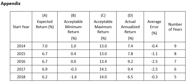
In all five cases we examined here, the average realized returns were inside the acceptable range. In addition, the average absolute error was just 1.4%. Taken together with the results from 2003 through 2013, all 16 cases had returns within the acceptable range and an average error of just 1.5%.
Larry Swedroe has authored or co-authored 18 books on investing. His latest is Your Essential Guide to Sustainable Investing. All opinions expressed are solely his opinions and do not reflect the opinions of Buckingham Strategic Wealth or its affiliates. This information is provided for general information purposes only and should not be construed as financial, tax or legal advice.


